I have two different Gene Ontology annotations for the genome annotation I am working with, and I’ve been trying different ways to quickly visualize Gene Ontology information, such as GO enrichment analysis using p-values as a proxy of significance (as per usual in genomic analyses). I thought of adapting this quick tutorial on wordcloud, but soon I noticed that sometimes the GO term human-readable descriptions are excruciatingly long, and the plots can become a total mess.

One option could be to inject a jumpline character after N words in the GO term string, which the R plotting engine seems to work fine with, but my first I thought was to abbreviate the words in the description. Perhaps unsurprised I learned that the foundational knowledge of R base has what I was looking for: the abbreviate() function.

Using some cheap tricks and workarounds to adapt to abbreviate()’s way of working, I made a function that returns abbreviated GO terms to pass to wordcloud(). Below is the script to do everything, with an example implemented in a loop to plot over different GO enrichment results plus a nice pretty picture of wordclouds and GO terms because we all love/hate wordclouds and GO terms.

Note: the loop assumes a number of different gene subsets (e.g. coming from your favorite clustering and/or differential expression methods), the order of which is the same for the different annotations (e.g.: “GOresults.BLAST2GO.1” is for the same genes as in “GOresults.eggNOG.1” ) .

# Install and load the packages I'll be using for this
install.packages("wordcloud")
library(wordcloud)
install.packages("RColorBrewer")
library(RColorBrewer)

# My data are in different independent tables, one per subset of genes. With this, I put them together as elements within a list, which facilitates iterating in for loops
pattern_b2go <- grep("allRes_blast2GO_elim",names(.GlobalEnv),value=TRUE)
list_b2go <- do.call("list",mget(pattern_b2go))

pattern_menogcur <- grep("allRes_menog1to1_cur_elim",names(.GlobalEnv),value=TRUE)
list_menogcur <- do.call("list",mget(pattern_menogcur))

# Some notes before following: The two important columns in these tables are "Term", which contains the GO term descriptions in human-readable format, and "classicFischer", the p-value of the Fisher test, a numeric value classically used to depict the level of significance (normally in -log(pvalue) format).

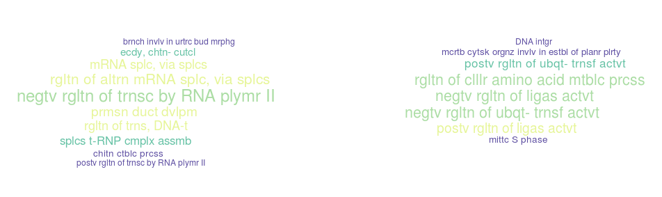
  # this first function abbreviates the GO term words to 5-letter words to make them easier to fit and display. Example: "negative regulation of transcription by RNA polymerase II" becomes "negtv rgltn of trnsc by RNA plymr II"
  abrevi <- function(x) { # The x argument is a character vector where every element is a human-readable GO term. 
    abr <- character() #empty vector where we'll dump every abbreviated GO term
    for (i in 1:length(x)) { # it will iterate over the number of elements in the x vector, i.e. the number of terms to be abbreviated
      a <- paste( # temporal placeholder for the newly abbreviated term. the idea is: split the GO term in every word, abbreviate separately, and put them back together with paste
        abbreviate(
          strsplit(x," ")[[i]], # the i-th element of the x vector of terms, split in every word separated by spaces
          minlength=5 # abbreviate for every word in the term to have a max of 5 letters
          ),
        collapse=" ") # the result of abbreviate is a vector with all the words. We put them back together using paste(..., collapse=" ")
      abr <- c(abr,a) # this adds the newly abbreviated term to the list of terms that will be returned
      }
    return(abr) # the list of abbreviated terms is returned
    }
  weirdscale <- function(x) { # this function transforms a set of numeric p-values to a readable scale that will allow to categorize them by color code and text size. Basically: relativize so that the min. value is 0 and the max is 100. Then, add +1.
    (-log(x)-min(-log(x)))/(max(-log(x))-min(-log(x)))*100+1
    }

for (i in 1:8){ # loop to plot my data
  b2go <- list_b2go[[i]] # grab GO results using BLAST2GO annotation for the i-th gene subset
  b2gonames <- b2go$Term[1:10] # character vector with the top-10 GO terms
  b2go_abr <- abrevi(b2gonames) # abbreviated terms as in the function above
  b2govalues <- as.numeric(b2go$classicFisher)[1:10] # make sure the pvalues are class numeric
  mnogC <- list_menogcur[[i]] # same for GO results using eggNOG annotation for the i-th gene subset
  mnogCnames <- menogC$Term[1:10]
  mnogC_abr <- abrevi(mnogCnames)
  mnogCvalues <- as.numeric(mnogC$classicFisher)[1:10]
  par(mfrow=c(1,2)) # set two plots per window, to see the same subset annotations side by side
  set.seed(10) # for reproducibility
  wordcloud( # the actual plot. first for the BLAST2GO annotation
    words = b2go_abr, # abbreviated GO terms
    freq = weirdscale(b2govalues), # their transformed, scaled values to be used as frequencies
    min.freq = 1,
    max.words = 200, # not used here as we use a top-10 list of terms
    random.order = FALSE,
    rot.per = 0, # frequency of rotated terms in the plot = 0 means all words will be horizontal
    colors = sample(brewer.pal(11, "Spectral"), 4), # grab 4 random colors from the 11-color palete "Spectral" of colorbrewer for color-coding the terms
    scale = c(1.5, 0.75) # min and max cex values for the terms
  )
  set.seed(10) # for reproducibility
  wordcloud(words= mnogC_abr, freq =weirdscale(mnogCvalues), min.freq = 1, max.words=200, random.order=FALSE, rot.per=0, colors=sample(brewer.pal(11, "Spectral"),4),scale=c(1.5,0.75)) # the same for eggNOG data
}

The result, for a given gene subset. Left is BLAST2GO and right is eggNOG. Some terms can be left reduced to undecipherable gibberish, but I think it works okay for the majority of them and for quick and simple visualizations.